Portfolio Projects

OBJECTIVE

1. Construct a risk-return optimized portfolio using the Markowitz Model.
2. Develop a written report determining the optimal portfolio and general rule of thumb.

---

GOALS

1. Demonstrate proficiency in the practical application of the Markowitz Model and Excel modeling.
2. Analyze the risk-return trade-off between different levels of risk aversion.
3. Explore various portfolios based on an array of hypothetical conditions.

---

DELIVERABLES

1. Dynamic Excel Workbook.
2. Written report (pasted in the report section below).

---

OVERVIEW

01 and 02 will not be part of our report. Only 03, 04, and 05 will be discussed below.
04 will consist of multiple portfolios based on various hypothetical scenarios.

---

DATA

Historical price: in Excel, use STOCKHISTORY() function to extract daily closing price
Dividend data: https://finance.yahoo.com/
Risk-Free Rate (10-year Treasury Rate): https://fred.stlouisfed.org/series/DGS10

The data spans from December 21, 2022, to December 21, 2023 (One entire year +1 day accounting for our calculating of daily return).

---

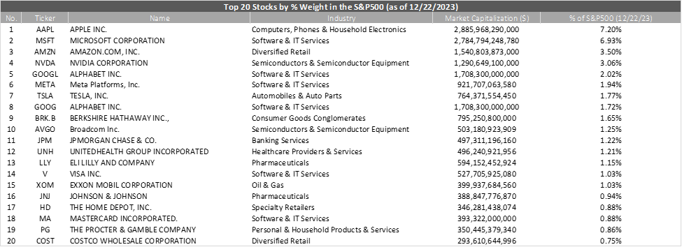
Company Selection

The companies that have been chosen are the top 20 companies by their weightage in the S&P500 for three main reasons: (1). Ample liquidity for rebalancing convenience and ease of construction, (2). The consistent positive performance of each company, and (3). Brand recognition establishes familiarity with the studied companies.

---

REPORT

03 Exploratory Analysis

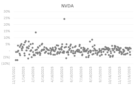
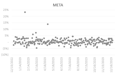
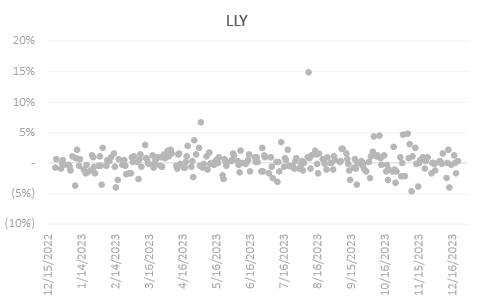
Generally, the data centers around 0.1% for all stocks. The tickers with the most significant outliers beyond the interquartile range are NVDA, META, TSLA, and LLY. The most dispersed tickers would be NVDA and TSLA, spanning between (7.15%) and (12.24%) to 24.37% and 11% respectively.

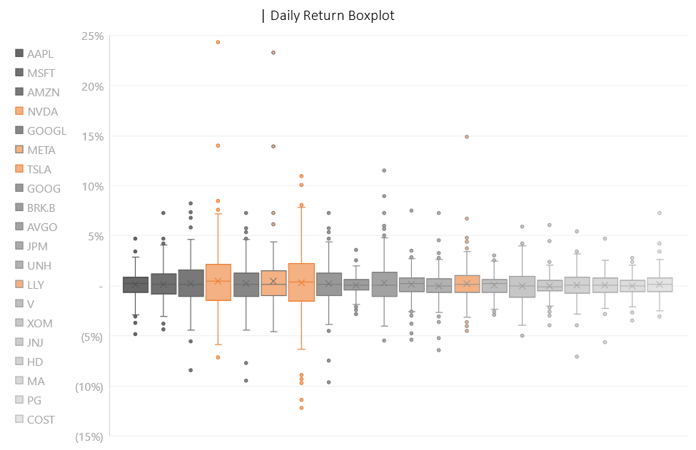
The two prominent returns beyond the interquartile range for NVDA were spotted in February—following NVAD’s favorable quarterly earnings announcement and an 8.6% EPS higher than expected, and May of 2023—following the same rally behind generative AI hype and beating expected earnings. For META, it was a bit earlier in the same two months of February and May. META on the other hand, after a tumultuous year and declining revenue, pledged to commit to business optimization and a $40 billion share repurchase plan during its quarterly earnings release, putting bullish pressure on the following month of February. TSLA on the other hand has sparse return data with no significantly isolated data points like the two above. Lastly, LLY has two significantly high returns, one in early May and another one in early August. It is wise to note that these market events generate abnormal returns but it is not important for our project as we do not intend to remove these data points from analysis at all.

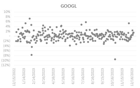
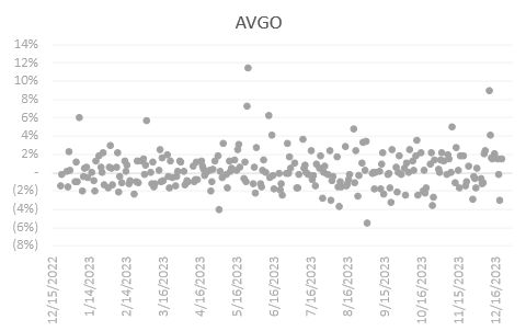
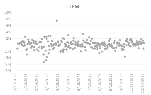
Zooming in the boxplot closer, most of the selected companies indicate normal distribution except AMZN, GOOGL, META, AVGO, and JPM. The only bank within the top 20 companies by weightage, JPM illustrated a negative skew the other significantly skewed stocks indicated the opposite direction of skewness.

AMZN shows generally sparse data points throughout the year with a few extremes in each fiscal quarter.

GOOGL has a positive outlook in the earlier months of 2023, having the majority of the returns above the 0% line with a narrowing trend moving toward the end of the year.

AVGO showed a bullish trend from mid-2023 onward with a lot of positive returns above the 0% line.

JPM demonstrated bearish sentiments during March of 2023, having numerous deep negative returns.

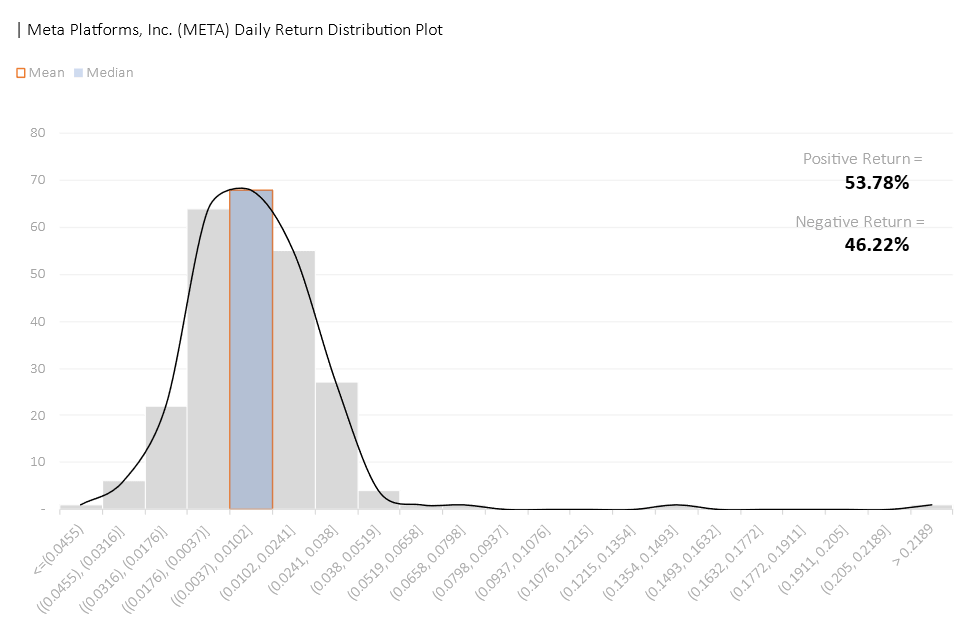
Amongst all 20 chosen stocks, NVDA has its return centered around the highest percentage with an average daily return of 0.48%. NVDA’s return is positive 56.18% of the time (within our studied period), falling behind COST of 58.57% with an average daily return of 0.15%, and JPM of 57.37% and an average daily return of 0.1%.

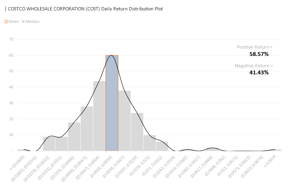
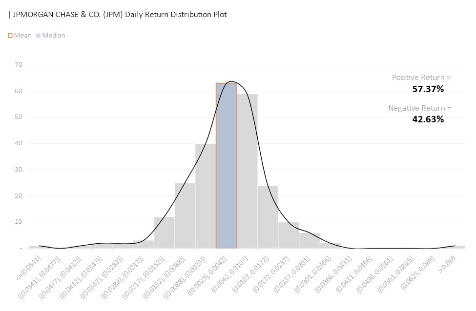
The company that offers the highest average daily return would be META with a mean daily return of 0.46%. However, only 53.78% of META’s returns are positive, approximately 4.78% behind COST, 3.59% behind JPM, and 2.39% behind NVDA.

We saw a considerable correlation between GOOGL and AMZN, GOOG and AMZN, META and GOOGL, META and GOOG, JPM and BRK.B, and MA and V. It was not surprising to see the tech giants having considerable collinearity as they operate under similar market conditions. Thus, we expect to see a diversified portfolio not consisting of both of the aforementioned pairs. The same goes for MA and V (Mastercard Incorporated and Visa Inc.).

One surprising correlation that we did not expect was JPM and BRK.B. We delved into the composition of BRK.B and found that BRK.B consists of over 9.03% of BAC (Bank of America Corp – as of September 30, 2023), a direct competitor to JPM. Therefore, we can rationalize this significant correlation given that a considerable component of BRK.B operates in the same space as JPM. It is important to note that while AMZN is also approximately 0.4% of BRK.B, we saw a weak correlation between the two prices, unlike V and MA.

Medium correlations can be observed between the following pairs of stock:

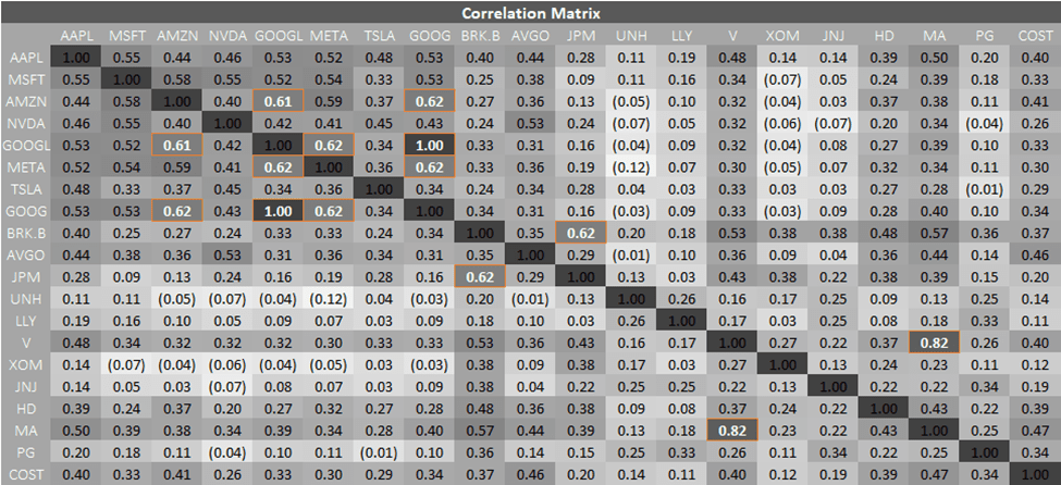
The correlations can be explained in a similar manner: (1). the tech companies operate in the same space and thus, are subjected to similar market pressure; and (2). BRK.B consists of less than 1% of each V and MA.

04 Portfolio Construction

04.1 Calculating the return

After setting up the table (calculating the daily return of each stock), we calculate the expected return of each security using the following formula:

And standard deviation or risk of each stock using the below formula:

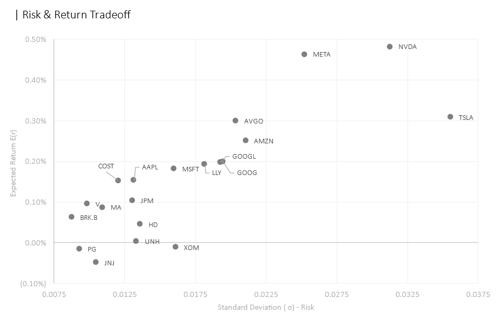
After calculating the expected return and standard deviation, we plotted each stock into the risk-return tradeoff space. The goal of our optimization process is to generate the combination that has the most favorable tradeoff, that is, a significant increase in expected return with minimal additional risk taken (visually speaking, a combination that resides in the upper left corner). We can expect a few stocks that would be in our portfolio because they are the closest to the upper left corner already such as COST, AAPL, MSFT, LLY, AVGO, META, and NVDA. Conversely, the opposite can be expected from those closest to the bottom right corner such as JNJ, XOM, and TSLA.

04.2 Setting Up the Portfolio

After that, we can assign dummy variables as the weight of each security like the following:

Then we can calculate our risky portfolio return, risky portfolio standard deviation, and Sharpe ratio using the formula below:

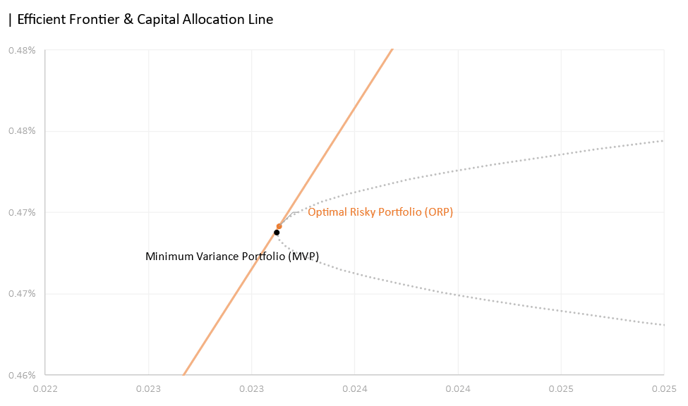
04.3 Optimizing the Portfolio

Within Excel, we use Solver to determine the optimal weightage for each stock for various simulations.

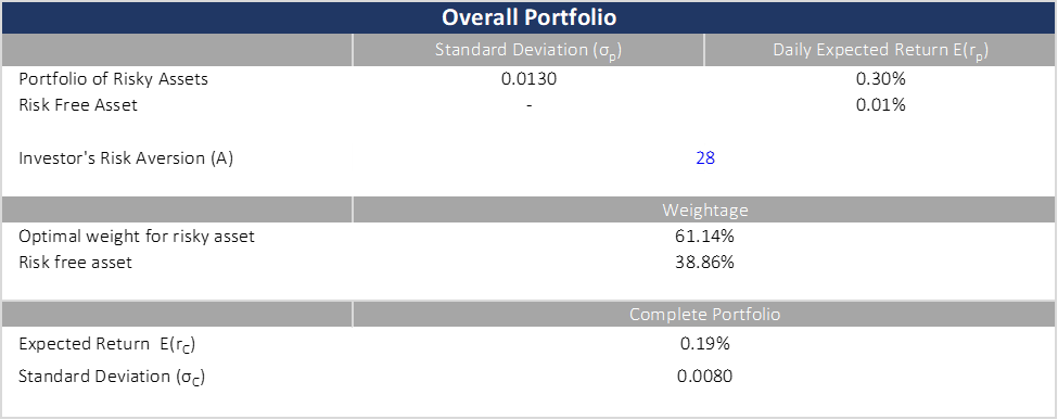
04.4 Calculating the Optimal % of Risky Asset

For the first iteration, we calculated the optimal percentage of risky assets based on a risk aversion coefficient A of 28, an average/modest risk tolerance for an investor. After that, we instead determined the investor’s risk aversion based on our target mix of risky assets and risk-free assets for comparison. With these iterations, we constructed various portfolios discussed below in 05.2. The optimal weight was calculated using the below formula:

Scenario 1: Only invests money at hand (1/3)

For this scenario, we use goal seek to maximize our Sharpe ratio, subjected to the following constraints:

1. We will only invest as much money as we have, that is, the sum of all asset weight (w_n) must be equal to 100%.
2. Each asset weight shall be between 0% and 100%, that is, less than or equal to 100% and greater or equal to 0%.

Scenario 2: allowing for 1.5X margin trade and short sell (2/3)

For this scenario, we use goal seek to maximize our Sharpe ratio, subjected to the following constraints:

1. The sum of all asset weight (w_n) must be equal to 100%.
2. Each asset weight can range between -150% and 150%, that is, less than or equal to 150% and greater or equal to 150%.

Scenario 3: A Simple portfolio of only two Risky assets (3/3)

1. The sum of all asset weight (w_n) must be equal to 100%.
2. Each asset weight shall be between 0% and 100%, that is, less than or equal to 100% and greater or equal to 0%.
3. We will only select two assets out of the twenty assets chosen.

05 Portfolio Comparison

05.1 Optimization Result

Portfolio 1 (1/3)

Below are the selected stock and the weightage of each security:

Portfolio 2 (2/3)

Below are the selected stock and the weightage of each security:

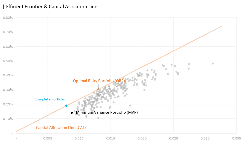
The efficient frontier was not able to be plotted due to computational power limitations.

Portfolio 3 (3/3)

Below are the selected stock and the weightage of each security:

• NVDA: 34.5%
• META: 65.5%

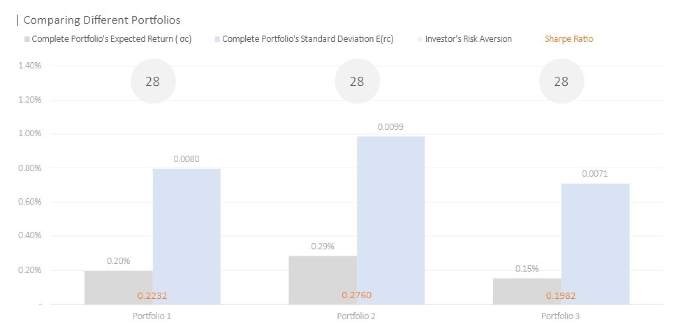
05.2 Comparing the results

We found at the same risk aversion, an investor benefitted the most from the second portfolio where all twenty assets are sold and purchased to construct a complete portfolio. The second portfolio provided a daily expected return 0.09% greater than the first portfolio without short selling. However, one should take note of the additional risk taken to improve the daily return. Additionally, constructing such a complex portfolio would take considerable effort to coordinate and maintain as well. Moreover, this is exclusive of the transaction costs involved. The third portfolio, despite its simplicity still provided a significant 15x improvement from the risk-free rate.

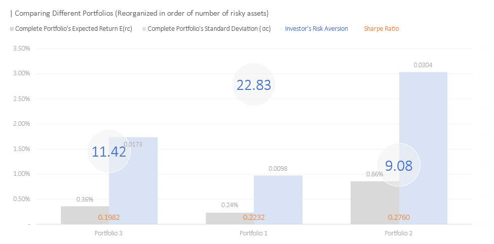
If we reorganize the portfolio in the order of number of assets, we can see that, the more diversified the portfolio, the better the expected return and Sharpe Ratio.

In terms of security selection, the anticipated stocks (stocks residing and along the border of the top left corner) are chosen for the first portfolio such as NVDA, META, AVGO, COST, and LLY. JPM was somewhat a surprise as we saw in the risk-return tradeoff space that it stood directly below AAPL—meaning that it offered inferior returns with the same amount of risk. The third portfolio indicated that the most efficient portfolio that consists of only two assets would be META and NVDA—the two assets with the highest expected daily return.

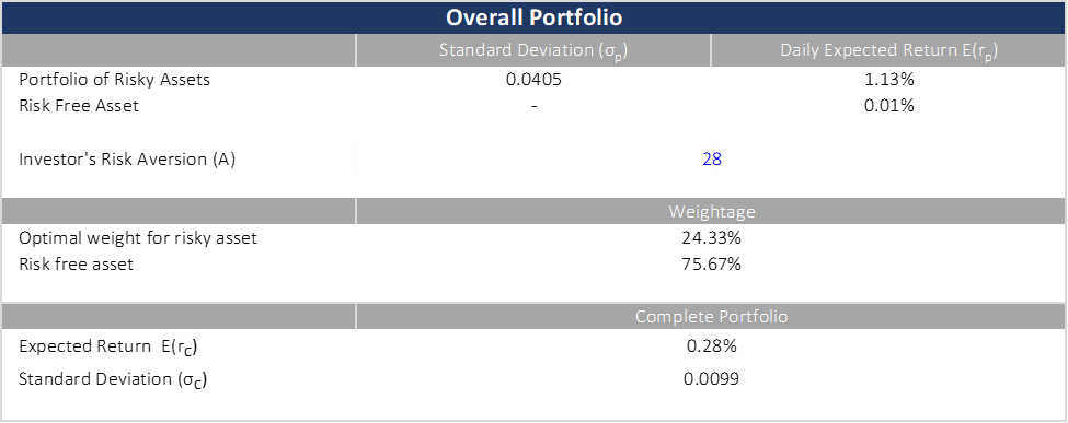
On the contrary, if we were to target our mix of risky assets and risk-free assets, we then get varying risk aversion instead.

We saw that at the same 75%-25% mix, the investor with the most diversified portfolio (portfolio 2) has the best Sharpe and expected daily return. The second-best Sharpe is the second most diversified portfolio (portfolio 1) followed by portfolio 3 with only two risky assets.

We saw a decline in the Sharpe Ratio from a 20 assets portfolio to 6 and to 2 assets. The Sharpe decline from Portfolio 2 to Portfolio 1 was a steep 0.0528 compared to a reduction of 0.025 from Portfolio 2 to Portfolio 1. Investor risk aversion on the other hand does not appear to coincide with the number of assets. Portfolio 1 has the riskiest investor—the highest risk coefficient of 22.83, with only 6 assets. The second most risky investor is Portfolio 3 followed by Portfolio 2.

Reorganizing the portfolio again based on the number of risky assets, we saw that the number of assets doesn’t necessarily correlate to better performance. Take note that the investor risk coefficient is now highest at portfolio 1 with six assets. It was unexpected initially but looking back at our model again, it was mechanically instructed to do so. What we did in portfolio 3 was basically selecting stocks that offered the highest daily expected return. Our Portfolio 1 chose 6 stocks: NVDA, META, AVGO, JPM, LLY, and COST; two of which are the entirety of Portfolio 3. In other words, portfolio 1 is portfolio 3 plus other relatively worse stocks that maximized our risk-return trade-off but unfortunately diminished our daily expected return. Regardless, we can see that the Sharpe Ration increases from left to right or with the increasing number of assets.

05.3 Conclusion

In sum, we can conclude that diversification often provides more resilience for a portfolio whether it is maximizing expected return or minimizing risk or the trade-off of both (maximizing Sharpe Ratio). As we saw in our first portfolio, the diversification only improved Sharpe with drawbacks to expected return. This is a flaw in the Markowitz model that we should consider. Additionally, from a data science point of view, our portfolio construction might be prone to data snooping bias because we only used a snapshot of all the stocks, not their entire performance history. Lastly, despite its simplicity, the Markowitz model quickly cracks when the number of assets increases. The computational power and complexity grew exponentially as we saw in portfolio 2 where we were unable to graph nor delve further like simpler portfolios.